
The Pivot Table is one of the most exciting Microsoft Excel features that allows you to organise your data easily. Pivot Table in Excel helps to calculate and analyse data to see comparisons and trends from a large data set.
After you finish this article, you will know how to create a Pivot Table in Excel, understand its significance, analyse business data properly and make effective business decisions for yourself or your organisation.
Never created a Pivot Table in Excel before? No worries, I will guide you throughout the article.
Firstly, you need to know what is the usage of Pivot Table.
Usage of the Pivot Table
The Pivot Table is one of the Excel features that initially looks difficult to use. But, once you get the hang of it, Pivot Tables gradually become really easy and useful.
Therefore, take a look at different scenarios where using the Pivot Table can prove to be convenient and useful.
Compare sales total
Imagine you have a worksheet that contains monthly sales data for three different products – X, Y and Z. Your task is to figure out which of these three products has been bringing the most money.
You can look through the worksheet and manually add the sales figure to a running total every time product X appears. You can do the same for product Y and Product Z until you have the total for all of them.
Now, imagine you have a monthly sales worksheet that has thousands and thousands of rows. Sorting them manually can take an entire lifetime. A Pivot Table can help you automatically aggregate all the sales figures for product X, product Y and product Z, as well as their respective sum, in a minute.
Show product sales as percentage of total sales
A Pivot Table normally shows the totals of each row or column as you create it but it’s not the only figure you can automatically produce.
Let us assume that you’ve entered quarterly sales numbers for product X, product Y, product Z into an Excel sheet and turned this data into a Pivot Table. The table would automatically give you three totals of each column.
What if you want to find the percentage these product sales contributed of all company sales instead of the sales totals?
With a Pivot Table, you can configure each column to give you the column’s percentage of all three column totals, instead of just the column total.
For instance, if product X, product Y, product Z totaled $100,000 in sales and the third product made $50,000, you can edit a pivot table to instead say this product contributed 2% of all company sales.
Simply right-click the cell carrying a sales total and select “Show Values As” > “% of Grand Total” to show product sales as percentages of total sales in a Pivot Table.
Combine duplicate data
Suppose, you’ve just completed a blog redesign where you had to update a bunch of URLs. Your blog reporting software didn’t handle it very well and ended up splitting the “view” metrics for single posts between two different URLs.
Now, in your spreadsheet, you have two separate instances of each individual blog post. In order to get accurate data, you need to combine the view totals for each of these duplicates.
Instead of having to manually search for and combine all the metrics from the duplicates, you can summarize your data with a Pivot Table. There you go! The view metrics from those duplicate blog posts will be aggregated automatically.
Get a head count
Pivot Tables are really helpful for calculating things automatically that you can’t easily do in a basic Excel table. An interesting feature is counting rows that all have something in common.
If you have a list of employees in an Excel sheet and next to their names are the respective departments they belong to, you can create a Pivot Table that shows you the number of employees in each of the departments.
Step By Step Guide to Create a Pivot Table in Excel
Here’s an infographic for a quick step by step guide to create a Pivot Table.
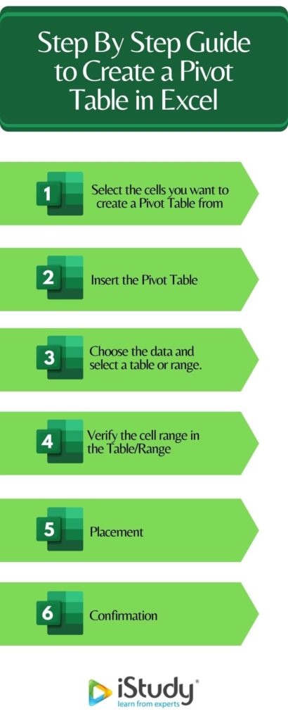
Step 1
The first step is about selecting the cells you want to create a Pivot Table from.
Every Pivot Table in Excel starts with a basic table. Enter your values into a specific set of rows and columns to create that table. The topmost row or topmost column should be used to categorize your values by what they represent.
It is to be noted that your data shouldn’t have any empty rows or columns. It must have only a single-row heading.
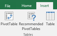
Step 2
The second step is to insert the Pivot Table.
You can create a Pivot Table from scratch or try the ones recommended in Microsoft Office.
Select Insert > PivotTable
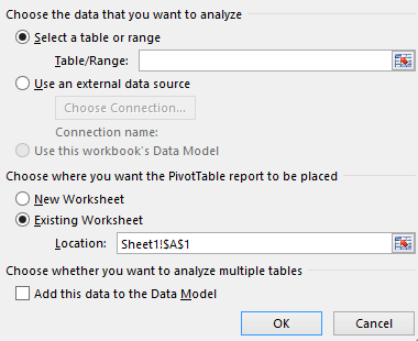
Step 3
For the third step, you need to choose the data you want to analyse and select a table or range.
Under Choose the data that you want to analyse, select, Select a table or range.
When you have entered all the data into your Excel sheet, you’ll want them to be in such a way that it’s easier to manage in a Pivot Table.
To sort your data, click the “Data” tab in the top navigation bar and select the “Sort” icon underneath it.
In the window that appears, you can sort your data by any column you want and in any order. If you want to sort your Excel sheet by “Total Sales”, for example, select the same column title under “Column” and then select whether you want the order to be from largest to smallest, or from smallest to largest.
Select “OK” on the bottom-right of the Sort window, and you’ll successfully reorder each row of your Excel sheet by the number of views each blog post has received.
Step 4
A range is a collection of cells in Microsoft Excel. 2 or more cells together make up a cell range. The fourth step is to verify the cell range in the Table/Range section.
The cells in a range shouldn’t necessarily be next to each other.
Step 5
The fifth step is about placement.
Under “Choose where you want the PivotTable report to be placed”, select New worksheet to place the Pivot Table in a new worksheet or Existing worksheet and then select the location you want the Pivot Table to appear.
Step 6.
The sixth and final step is about confirmation.
Once you have everything in place, click OK.
How to build a Pivot Table in Excel
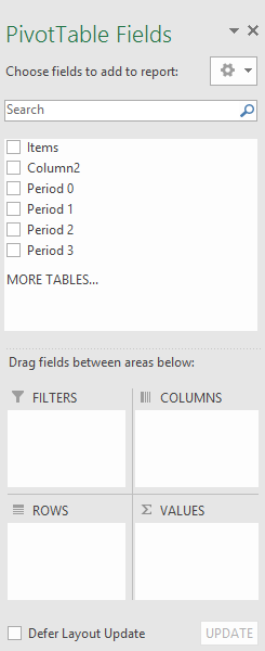
In order to add a field to your PivotTable, select the field name checkbox in the PivotTables Fields pane.
It is to be noted that selected fields are added to their default areas: non-numeric fields are added to Rows, date and time hierarchies are added to Columns, and numeric fields are added to Values. If you want to move a field from one area to another, just drag the field to the target area.
Conclusion
If you’re still reading this, you have by now learned the basics of creating a Pivot Table in Excel. However, depending on your nature of work and your need for a Pivot Table, you might not be done yet.
iStudy offers a comprehensive course that encompasses beginner, intermediate and advanced levels of Microsoft Excel. This accredited all-you-need-to-know course will help you to extensively learn every aspect of Microsoft Excel.
The use and importance of Microsoft Excel is only increasing every day. It is gradually establishing itself as an indispensable tool in day to day administrative activities. It is only a matter of time until it becomes a skill that is going to give an edge to anyone in the competitive job market.

Hey, thanks for the article post. Much thanks again. Really Cool. Darcey Sloane Shelman
Good job. Thanks for sharing nice tips to link exchange. Anna-Diana Frederik Carroll
Fantastic blog article. Thanks Again. Really Great. Biddy Had Stuart Keeley Bogey Sunderland
I was excited to uncover this site. I want to to thank you for ones time for this particularly fantastic read!! I definitely liked every part of it and i also have you saved as a favorite to check out new stuff in your blog. Aubrie Hermon Petite
I have learn some excellent stuff here. Certainly value bookmarking for revisiting. I surprise how much effort you place to create any such magnificent informative site.| Carmina Kendell Rem
I believe you have noted some very interesting details, thanks for the post. Marlo Sayres Ahouh
I really like looking through an article that can make people think. Also, thank you for permitting me to comment! Sydelle Todd Ashlen
Nice blog here! Also your site loads up very fast! Rhianna Budd Lek
Really enjoyed this blog post. Thanks Again. Want more. Maribeth Josh Sheffie
I am extremely impressed together with your writing abilities as well as with the format on your blog. Is that this a paid topic or did you customize it your self? Either way stay up the excellent quality writing, it is rare to look a nice blog like this one these days..| Blinnie Yardley Kalinda
I truly prize your piece of content, Terrific post. Jemmy Vinny Desma
Thanks so much for the blog post. Thanks Again. Great. Trude Wallas Kama
There is definately a lot to know about this topic. I love all of the points you have made. Saidee Brodie Natelson
Hello there. I found your website by means of Google even as searching for a related topic, your website got here up. It appears to be great. I have bookmarked it in my google bookmarks to come back then. Nerti Nathanial Pricilla
Very true Sally. Thank you for putting so eloquently. Nani Salmon Rahal
Hi my friend! I wish to say that this post is awesome, great written and come with almost all important infos. Phoebe Andie Geof